
Introduction
A stationary process is a fundamental concept in time series analysis. A time series is said to be stationary if its statistical properties—such as mean, variance, and autocorrelation—do not change over time. Understanding stationarity is crucial because many statistical and machine learning models assume that the data is stationary.
In this tutorial, we will cover:
- What a stationary process is
- Types of stationarity
- How to check for stationarity
- Transformations to achieve stationarity
- Practical implementation using Python
1. What is a Stationary Process?
A stationary process is a stochastic process whose statistical properties remain constant over time. This means that:
- The mean remains the same over time.
- The variance is constant (homoscedasticity).
- The autocovariance (correlation with past values) depends only on the time lag and not on time itself.
Mathematically, a time series Xt is strictly stationary if, for any time points t1, t2,...,tn and any time shift h:
P(Xt1, Xt2,..., Xtn) = P(Xt1+h, Xt2+h, ...,Xtn+h)
This means the probability distribution remains unchanged over time.
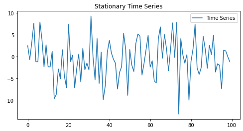
Example of a Stationary Process
Consider a white noise process:
Xt = et, where et ~ N(0,s2)
This is stationary because its mean is zero, variance is constant, and there is no correlation between values.
 Download Python Code
2. Types of Stationarity
There are different degrees of stationarity.
a) Strict Stationarity
A process is strictly stationary if the joint probability distribution does not change with time shifts. This is a strong requirement and is rarely used in practical applications.
P(Xt1, Xt2,..., Xtn) = P(Xt1+h, Xt2+h, ...,Xtn+h) where h is any arbitratry time lag
b) Weak (Second-Order) Stationarity
A process is weakly stationary if:
- The mean is constant over time:
E[Xt] = E[Xt+h] = µ.
- The variance is finite and constant:
Var(Xt) = Var(Xt+h) = s2
- The autocovariance depends only on the lag h, not on time t:
Cov(Xt, Xt+h) = Y(h)
Many time series models, such as ARMA and ARIMA, assume weak stationarity.
c) Trend Stationarity vs. Difference Stationarity
- Trend Stationary: The time series has a deterministic trend that can be removed (e.g., by detrending).
- Difference Stationary: The series can be made stationary by differencing (e.g., first-order differencing: Xt - Xt-1).
3. How to Check for Stationarity?
There are several ways to check if a time series is stationary.
a) Visual Inspection
Plot the time series and look for:
- A changing mean (non-stationary)
- Increasing or decreasing variance (non-stationary)
- Cyclical patterns (could indicate seasonality)

Download Python Code
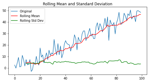
b) Rolling Statistics
Calculate the rolling mean and rolling standard deviation. If they change over time, the series is non-stationary.
Download Python Code
c) Augmented Dickey-Fuller (ADF) Test
The ADF test is a statistical test where the null hypothesis is that the series has a unit root (i.e., it is non-stationary). If the p-value is below a significance level (e.g., 0.05), we reject the null hypothesis, indicating stationarity.
Download Python Code
d) Kwiatkowski-Phillips-Schmidt-Shin (KPSS) Test
The KPSS test has the opposite hypothesis: the null hypothesis is that the series is stationary. If the p-value is below 0.05, we reject the null hypothesis, meaning the series is non-stationary.
Download Python Code
4. Making a Non-Stationary Series Stationary
If the series is non-stationary, we can apply transformations to make it stationary.
a) Differencing
Subtract the previous value from the current value and check for stationarity again using ADF.

Download Python Code
b) Log Transformation
Reduces heteroscedasticity (changing variance).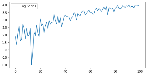
Download Python Code
c) Detrending
Remove the trend component.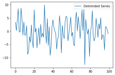
Download Python Code
5. Practical Example: Real-World Data
Let's use stock prices (which are usually non-stationary) and apply stationarity techniques. If the ADF p-value is below 0.05 after differencing, we have achieved stationarity.